Yangyehan&UndGround.

Embedding And Dense Retrieval

Word count: 2.8kReading time: 14 min
2024/02/07

Embeddings And Dense Retrieval

1
2
3
4
# cohere 是一个NLP的库,提供了embedding的函数
# cohere 官网:https://cohere.com/
# umap-learn,altair 是一个统计可视化库,在后面,我们会使用它来可视化embedding数据的二维空间位置
# !pip install cohere umap-learn altair datasets
1
2
3
4
import cohere
api_key = 'pyRCp2X2I9sB07zO5050dG9qJ1tHinT1fYbSCBO9'
co = cohere.Client(api_key)
import numpy as np
1
import pandas as pd

Word Embeddings

Embeddings.png

Consider a very small dataset of three words

1
2
3
4
5
6
7
three_words = pd.DataFrame({'text':
[
'joy',
'happiness',
'potato'
]})
three_words

image-20240207024121991

Let’s create the embedding for the three words

1
2
# list(),将对象转换成列表
list(three_words['text'])
['joy', 'happiness', 'potato']
1
2
three_words_emb = co.embed(texts = list(three_words['text']),model = 'embed-english-v2.0').embeddings
type(three_words_emb)
list
1
2
3
word_1 = three_words_emb[0]
word_2 = three_words_emb[1]
word_3 = three_words_emb[2]
1
word_1[:5]
[2.3203125, -0.18334961, -0.578125, -0.7314453, -2.2050781]

Sentence Embedding

Consider a very small dataset of three sentence

1
2
3
4
5
6
7
8
9
10
11
12
13
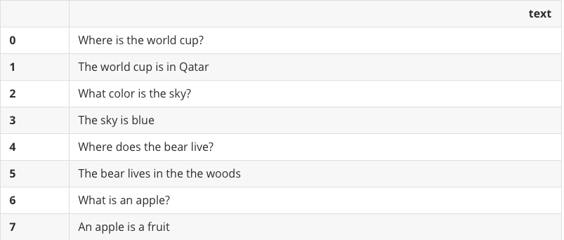
sentences = pd.DataFrame({
'text':[
'Where is the world cup?',
'The world cup is in Qatar',
'What color is the sky?',
'The sky is blue',
'Where does the bear live?',
'The bear lives in the the woods',
'What is an apple?',
'An apple is a fruit',
]
})
sentences

image-20240207023949056

create embeddings

1
2
3
4
5
emb = co.embed(texts=list(sentences['text']),model ='embed-english-v2.0').embeddings

# 查看10个句子中每个向量的前三个数据
for e in emb:
print(e[:3])
[0.27319336, -0.37768555, -1.0273438]
[0.49804688, 1.2236328, 0.4074707]
[-0.23571777, -0.9375, 0.9614258]
[0.08300781, -0.32080078, 0.9272461]
[0.49780273, -0.35058594, -1.6171875]
[1.2294922, -1.3779297, -1.8378906]
[0.15686035, -0.92041016, 1.5996094]
[1.0761719, -0.7211914, 0.9296875]
1
len(emb[0])
4096
1
2
3
4
5
6
7
8
9
10
11
12
13
14
15
16
17
18
19
20
21
22
23
24
25
26
27
28
29
30
31
32
33
34
35
36
37
38
39
40
41
42
43
44
45
46
47
48
49
50
51
52
53
54
55
56
57
58
59
60
61
62
63
64
65
66
67
68
69
70
71
72
73
74
75
76
77
78
79
80
81
82
83
84
85
86
87
88
89
90
91
92
93
94
95
96
97
98
99
100
101
102
103
104
105
106
107
108
109
# Sentences embedding后的可视化脚本
import umap
import altair as alt

from numba.core.errors import NumbaDeprecationWarning, NumbaPendingDeprecationWarning
import warnings

warnings.simplefilter('ignore', category=NumbaDeprecationWarning)
warnings.simplefilter('ignore', category=NumbaPendingDeprecationWarning)


def umap_plot(text, emb):

cols = list(text.columns)
# UMAP reduces the dimensions from 1024 to 2 dimensions that we can plot
reducer = umap.UMAP(n_neighbors=2)
umap_embeds = reducer.fit_transform(emb)
# Prepare the data to plot and interactive visualization
# using Altair
#df_explore = pd.DataFrame(data={'text': qa['text']})
#print(df_explore)

#df_explore = pd.DataFrame(data={'text': qa_df[0]})
df_explore = text.copy()
df_explore['x'] = umap_embeds[:,0]
df_explore['y'] = umap_embeds[:,1]

# Plot
chart = alt.Chart(df_explore).mark_circle(size=60).encode(
x=#'x',
alt.X('x',
scale=alt.Scale(zero=False)
),
y=
alt.Y('y',
scale=alt.Scale(zero=False)
),
tooltip=cols
#tooltip=['text']
).properties(
width=700,
height=400
)
return chart

def umap_plot_big(text, emb):

cols = list(text.columns)
# UMAP reduces the dimensions from 1024 to 2 dimensions that we can plot
reducer = umap.UMAP(n_neighbors=100)
umap_embeds = reducer.fit_transform(emb)
# Prepare the data to plot and interactive visualization
# using Altair
#df_explore = pd.DataFrame(data={'text': qa['text']})
#print(df_explore)

#df_explore = pd.DataFrame(data={'text': qa_df[0]})
df_explore = text.copy()
df_explore['x'] = umap_embeds[:,0]
df_explore['y'] = umap_embeds[:,1]

# Plot
chart = alt.Chart(df_explore).mark_circle(size=60).encode(
x=#'x',
alt.X('x',
scale=alt.Scale(zero=False)
),
y=
alt.Y('y',
scale=alt.Scale(zero=False)
),
tooltip=cols
#tooltip=['text']
).properties(
width=700,
height=400
)
return chart

def umap_plot_old(sentences, emb):
# UMAP reduces the dimensions from 1024 to 2 dimensions that we can plot
reducer = umap.UMAP(n_neighbors=2)
umap_embeds = reducer.fit_transform(emb)
# Prepare the data to plot and interactive visualization
# using Altair
#df_explore = pd.DataFrame(data={'text': qa['text']})
#print(df_explore)

#df_explore = pd.DataFrame(data={'text': qa_df[0]})
df_explore = sentences
df_explore['x'] = umap_embeds[:,0]
df_explore['y'] = umap_embeds[:,1]

# Plot
chart = alt.Chart(df_explore).mark_circle(size=60).encode(
x=#'x',
alt.X('x',
scale=alt.Scale(zero=False)
),
y=
alt.Y('y',
scale=alt.Scale(zero=False)
),
tooltip=['text']
).properties(
width=700,
height=400
)
return chart
1
chart = umap_plot(sentences, emb)
1
chart.interactive()

Pasted Graphic 6.png

Articles Embedding

1
2
3
import pandas 
wiki_articles = pd.read_pickle('wikipedia.pkl')
wiki_articles

image.png

1
import numpy as np
1
2
3
4
5
6
#[[]] 在pandas中表示有多列被选中
articles = wiki_articles[['title', 'text']]

# 便利wiki_articles数据中的每一行的emb元素存储在第一个d中,d表示每一行的['emb']是一个二维向量数组,再次便利每一个emb中的每一个向量元素,存储在第二个d中
# 并使用np.array将其转换为二维数组
embeds = np.array([d for d in wiki_articles['emb']])
1
# articles

image.png

1
type(wiki_articles['emb'])
pandas.core.series.Series
1
2
chart = umap_plot_big(articles, embeds)
chart.interactive()

image.png

接下来我们来一起看一个例子

Dense Retrieval.png

1
2
3
4
5
# AnnoryIndex  ANN(Aproximate Nearest Neighbors,ANN) 近似最邻近搜索
from annoy import AnnoyIndex
import numpy as np
import pandas as pd
import re
1
2
3
4
5
6
7
8
9
10
11
12
13
14
15
16
17
text = """
Interstellar is a 2014 epic science fiction film co-written, directed, and produced by Christopher Nolan.
It stars Matthew McConaughey, Anne Hathaway, Jessica Chastain, Bill Irwin, Ellen Burstyn, Matt Damon, and Michael Caine.
Set in a dystopian future where humanity is struggling to survive, the film follows a group of astronauts who travel through a wormhole near Saturn in search of a new home for mankind.

Brothers Christopher and Jonathan Nolan wrote the screenplay, which had its origins in a script Jonathan developed in 2007.
Caltech theoretical physicist and 2017 Nobel laureate in Physics[4] Kip Thorne was an executive producer, acted as a scientific consultant, and wrote a tie-in book, The Science of Interstellar.
Cinematographer Hoyte van Hoytema shot it on 35 mm movie film in the Panavision anamorphic format and IMAX 70 mm.
Principal photography began in late 2013 and took place in Alberta, Iceland, and Los Angeles.
Interstellar uses extensive practical and miniature effects and the company Double Negative created additional digital effects.

Interstellar premiered on October 26, 2014, in Los Angeles.
In the United States, it was first released on film stock, expanding to venues using digital projectors.
The film had a worldwide gross over $677 million (and $773 million with subsequent re-releases), making it the tenth-highest grossing film of 2014.
It received acclaim for its performances, direction, screenplay, musical score, visual effects, ambition, themes, and emotional weight.
It has also received praise from many astronomers for its scientific accuracy and portrayal of theoretical astrophysics. Since its premiere, Interstellar gained a cult following,[5] and now is regarded by many sci-fi experts as one of the best science-fiction films of all time.
Interstellar was nominated for five awards at the 87th Academy Awards, winning Best Visual Effects, and received numerous other accolades"""

Split into Chunks

1
2
3
4
5
texts = text.split('.')

# remove the /n for every sentence
texts = [t.strip('\n') for t in texts]
texts
['Interstellar is a 2014 epic science fiction film co-written, directed, and produced by Christopher Nolan',
 'It stars Matthew McConaughey, Anne Hathaway, Jessica Chastain, Bill Irwin, Ellen Burstyn, Matt Damon, and Michael Caine',
 'Set in a dystopian future where humanity is struggling to survive, the film follows a group of astronauts who travel through a wormhole near Saturn in search of a new home for mankind',
 'Brothers Christopher and Jonathan Nolan wrote the screenplay, which had its origins in a script Jonathan developed in 2007',
 'Caltech theoretical physicist and 2017 Nobel laureate in Physics[4] Kip Thorne was an executive producer, acted as a scientific consultant, and wrote a tie-in book, The Science of Interstellar',
 'Cinematographer Hoyte van Hoytema shot it on 35 mm movie film in the Panavision anamorphic format and IMAX 70 mm',
 'Principal photography began in late 2013 and took place in Alberta, Iceland, and Los Angeles',
 'Interstellar uses extensive practical and miniature effects and the company Double Negative created additional digital effects',
 'Interstellar premiered on October 26, 2014, in Los Angeles',
 'In the United States, it was first released on film stock, expanding to venues using digital projectors',
 'The film had a worldwide gross over $677 million (and $773 million with subsequent re-releases), making it the tenth-highest grossing film of 2014',
 'It received acclaim for its performances, direction, screenplay, musical score, visual effects, ambition, themes, and emotional weight',
 'It has also received praise from many astronomers for its scientific accuracy and portrayal of theoretical astrophysics',
 ' Since its premiere, Interstellar gained a cult following,[5] and now is regarded by many sci-fi experts as one of the best science-fiction films of all time',
 'Interstellar was nominated for five awards at the 87th Academy Awards, winning Best Visual Effects, and received numerous other accolades']

Get Embeddings

1
2
3
4
5
6
# Get Embeddings
response= co.embed(texts = texts).embeddings
# embed 是一个二维数组
# 这里将其转换为一个数组,主要是为了方便后面获取嵌入向量的特征维度
embeds = np.array(response)
embeds.shape
(15, 4096)

Create Search_index

在写代码之前这里先简单介绍一下构建ANN_search_index的原理,以及ANN工作原理:

近似最近邻(Approximate Nearest Neighbor, ANN)算法的核心目标是在高维空间中快速找到与给定查询点最接近的数据点,而不需要进行精确的最近邻搜索。由于高维空间的复杂性,直接进行精确搜索通常是计算成本极高的。ANN算法通过构建一种近似的数据结构来实现这一目标,这种数据结构能够在保持一定搜索精度的同时,显著提高搜索效率。

ANN构建索引的原理通常基于以下几个关键概念:

  1. 局部敏感哈希(Locality Sensitive Hashing, LSH)
    LSH是一种将相似项映射到相同哈希桶的技术。通过这种方式,相似的数据点在哈希空间中更有可能被分配到相同的桶中。Annoy库使用LSH作为其核心算法之一,通过构建多个哈希表来组织数据点。

  2. 树结构
    Annoy库使用树状结构(如KD树、球树等)来组织数据点。在构建索引时,这些树会根据数据点的特征进行分割,形成层次结构。查询时,算法会沿着树的路径进行搜索,以找到最接近的邻居。

  3. 随机投影
    为了减少高维数据的维度,Annoy使用随机投影来创建数据点的低维表示。这些投影保留了数据点之间的相对距离,使得相似的数据点在投影后仍然保持接近。

  4. 并行搜索
    Annoy通过构建多棵树并行搜索来提高搜索效率。每棵树都是独立的,可以并行处理查询,从而减少整体的搜索时间。

ANN的工作原理大致如下:

  1. 索引构建

    • 数据点首先被添加到索引中,每个数据点都会被分配到一个或多个哈希桶中。
    • 然后,Annoy会构建多棵树,每棵树都包含数据点的投影。
    • 在构建过程中,Annoy会优化树的结构,以确保搜索时能够快速地找到最接近的邻居。
  2. 查询

    • 当需要查询最近邻时,Annoy会将查询点投影到相同的哈希桶和树结构中。
    • 对于每棵树,算法会从根节点开始,根据查询点的特征值沿着树向下搜索,直到找到最接近的邻居。
    • 由于有多个树,Annoy会收集所有树的结果,并合并它们以得到最终的最近邻列表。
  3. 结果优化

    • 在搜索过程中,Annoy可能会使用一些启发式方法来优化结果,例如,通过限制搜索的深度或节点数量来平衡搜索速度和精度。

通过这种方式,ANN能够在保持较高搜索精度的同时,显著提高搜索速度,使其适用于大规模数据集和实时应用场景。

这里稍微补充一下这个基于树构建索引,实际上就是提前在高维空间,将数据划分区块,通过数据点与垂直向量做内积的方式,将区块划分左子树还是又子树来构建树,这样在后面查询的时候,首先通过树来找到区域,再到这个区域里做近似最邻近搜索(ANN)

1
2
3
4
5
6
7
8
9
10
11
12
13
14
15
# 创建索引 两个参数:当个数据点的特征维度(索引维度),计算方法
search_index = AnnoyIndex(embeds.shape[1],'angular')

# 将所有的嵌入向量添加到索引中
# 这里的embed是一个二维数组,embed[i]表示第i行
# 这里search_index存的并不是真正的文本而是文本在texts里的index和embeddings
# 所以会直接导致后面similar_item_ids返回的是文本在texts里的index
for i in range(len(embeds)):
search_index.add_item(i, embeds[i])

# 构建树
search_index.build(10)
# 保存创建的索引,对于相同的数据下次搜索的时候,不用重复创建索引
search_index.save('test.ann')

True
1
2
3
4
5
6
7
8
9
10
11
12
13
14
15
16
17
18
19
20
21
22
23
pd.set_option('display.max_colwidth', None)

def search(query):

# Get the query's embedding
query_embed = co.embed(texts=[query]).embeddings

# Retrieve the nearest neighbors
similar_item_ids = search_index.get_nns_by_vector(query_embed[0],
3,
include_distances=True)

# Format the results
# similar_item_ids 返回的其实texts的index和distance
results = pd.DataFrame(data={'texts': [texts[t] for t in similar_item_ids[0]],
'distance': similar_item_ids[1]})

# 创建json格式输出
json = []
for i in range(len(similar_item_ids[0])):
json.append({'text':texts[i],'distence':similar_item_ids[1][i]})

return results,json
1
2
3
query="How much did the film make?"
result,json = search(query)
result

image.png

CATALOG
  1. 1. Embeddings And Dense Retrieval
    1. 1.0.1. Word Embeddings
    2. 1.0.2. Sentence Embedding
  2. 1.1. Articles Embedding
  3. 1.2. 接下来我们来一起看一个例子
    1. 1.2.1. Build vector database and use Dense Search
    2. 1.2.2. Split into Chunks
    3. 1.2.3. Get Embeddings
    4. 1.2.4. Create Search_index
    5. 1.2.5. 在写代码之前这里先简单介绍一下构建ANN_search_index的原理,以及ANN工作原理:
    6. 1.2.6. 到此我们就做了一个Vector database,并使用基于ANN的Dense Search